2012 Annual Science Report
 University of Wisconsin
Reporting | SEP 2011 – AUG 2012
University of Wisconsin
Reporting | SEP 2011 – AUG 2012
Project 3C: In Situ Fe Isotope Analysis of Iron Formations
Project Summary
The Fe isotope composition of magnetite from the oldest (~3.8 Ga) sedimentary banded iron formations of Isua Greenland provide important constraints on the amount of Fe oxidation and its possible pathways. Iron isotope compositions of individual magnetite layers have been measured at the millimeter scale by micromilling and conventional mass spectrometry analysis and at the micrometer scale using femtosecond laser ablation (fs-LA). There is limited variability in the iron isotope composition of magnetite within a layer as would be expected for these amphibolites grade rocks. Within an individual hand sample there is at most a 0.3 ‰ difference in δ56Fe values between different layers. Over a scale of tens of kilometers, the δ56Fe values between magnetite layers in different samples range from +1.1 to +0.4 ‰. These high positive δ56Fe values are noteworthy, and as a whole, Isua iron formations have higher and less variable δ56Fe values as compared to the more massive 2.5 Ga iron formations from the Hamersley basin in Australia and the Transvaal basin in South Africa. This contrast in measured Fe isotope composition is best interpreted as having been produced by differing pathways of Fe cycling. The Isua BIFs most likely formed by small amounts of Fe oxidation from a water column caused by anoxygenic phototrophs with limited diagenetic alteration, whereas the younger 2.5 Ga Australian and South African BIFs were most likely formed by higher proportions of Fe oxidation and considerable diagenetic reactions that took place between pore fluids and iron oxide gels
Project Progress
The oldest well preserved sedimentary rocks are the 3.8 to 3.7 billion year old Isua supracrustal sequences in Greenland. Because these rocks recorded the surficial environmental conditions in which they were deposited, these rocks have been the subject of extensive geological and geochemical investigation to infer past biological activity and atmospheric conditions (e.g., Schidlowski et al., 1979; Rosing, 1999; Rosing and Frei, 2004). Banded iron formations also occur in this sequence of sedimentary rocks and their presence indicates that there was enough oxidant present to oxidize and precipitate ferrous iron from solution. Iron isotope investigations of these iron formations have concluded that the Fe isotope compositions are not a result of the greenschist/amphibolites grade metamorphism and that in general the Fe isotope compositions are consistent with only partial Fe oxidation of Fe derived from hydrothermal fluids (Dauphas et al., 2004; 2007; Whitehouse and Fedo, 2007). However, in a microscale study that used Secondary Ionization Mass Spectrometry (SIMS) to measure the Fe isotope composition of magnetite from Isua BIF’s, Whitehouse and Fedo (2007) found large ~2 ‰ variations of magnetite grains that are tens of μm apart and suggested that magnetite with high δ56Fe values (up to 2 ‰) represent partial oxidation of ferrous fluids and that magnetite grains with lower δ56Fe values, as low as -1 ‰, were formed by exchange with pore fluids that had low δ56Fe values from which the magnetite inherited its low δ56Fe values. The implication of these presumed reservoir effects are that there was evidence for dissimilatory Fe reducing bacteria to produce fluids with low δ56Fe values or that there was sufficient amounts of an oxidant present in the sediment gel to oxidize aqueous Fe(II) trapped as pore fluids which results in fluids with low δ56Fe values.
We have undertaken an Fe isotope study of Isua iron formation rocks that includes analysis of Fe isotope variations at the tens of kilometers scale based on analysis of hand samples, at the millimeter scale based on micromilling and analysis by solution nebulization, and at the micrometer scale by use of femtosecond laser ablation (fs-LA). Overall, the Fe isotope composition of the magnetite layers from the 7 hand samples analyzed in this study, δ56Fe values ranged from 0.4 to 1.1 ‰ providing evidence for Fe isotope variability at the kilometer scale range. In contrast, at the hand sample scale there was limited variability both within a magnetite layer and between magnetite layers in the same hand sample. Micromilled samples were typically obtained from an area that was 2 × 2 × 0.1 mm in size and for most samples there was no measureable Fe isotope variability within a layer. For example, 7 of the 10 layers that had more than 1 micromilled sample spot in a single layer, had a magnetite layer range in δ56Fe values less than 0.13 ‰, which is the 2-σ external error for our analytical method. Three layers defined minor Fe isotope variability with a range of δ56Fe values of between 0.18 and 0.26 ‰. Analysis using fs-LA analysis on spots that were 60 × 40 × 6 μm show no isotope variability within a layer given the external 2-σ precision of our fs-LA protocol, which is ±0.2 ‰ in 56Fe/54Fe. For layers sampled by both micromilling and fs-LA, agreement in measured 56Fe/54Fe ratios was excellent indicating that the fs-LA method is accurate. Figure 1 shows a representative sample that was micromilled and analyzed by fs-LA.
The lack of significant Fe isotope variability within a magnetite layer is consistent with the metamorphic conditions that these samples have experienced where diffusion calculations indicate that Fe would completely diffuse over the 2 mm length of our micromilling in 3 million years and over the 60 μm length of our fs-LA raster areas in 0.3 million years and thus one would not expect to measure Fe isotope variability within a layer. In contrast, interlayer variability is expected because Fe diffusion across the silicates that separate magnetite layers would be much slower and this is what we observe in the micromilled and fs-LA analyses. The origin of the significant variability found by the Whitehouse and Fedo (2007) study is unknown. Although our samples came from the same low strain area as the samples studied by Whitehouse and Fedo (2007), we have not analyzed the same samples and thus any discussion of the reason why our findings and theirs are different is challenging. However, we note that significant mass dependent fractionation for both O and Fe isotope analyses on magnetite have been found during analysis by SIMS that is associated with the angle between the primary ion beam and the magnetite crystal lattice (Huberty et al., 2010; Kita et al., 2011; Lyon et al., 1998) and we suggest that the significant range of Fe isotope compositions measured by Whitehouse and Fedo (2007) may in part represent an analytical artifact associated with mineral orientation with respect to the primary ion beam in a SIMS analysis.
Magnetite formation in BIFs is largely a result of Fe(II) oxidation to a hydrous ferric oxide (HFO) precipitate followed by reaction of the HFO with aqueous Fe(II) to produce the mixed valence state Fe3O4. For the case of limited interaction with Fe(II), the δ56Fe of magnetite will be driven by the mixing relationship of:
δ56FeMt = ⅔ δ56FeHFO + ⅓ δ56FeFe(II)aq.
In contrast, if there is significant Fe(II) exchange with magnetite the δ56Fe of the magnetite will be governed by the δ56Fe of Fe(II) and the equilibrium fractionation factor between magnetite–Fe(II)aq which is Δ56Femt-Fe(II) = 2.2 ‰ based on the β56/54 values for Fe(II)aq from Rustad et al. (2010) and magnetite from Polyakov et al. (2007), which are the preferred formulations based on agreement between experimental investigations of Fe(II)aq–mineral fractionations (Beard et al., 2010). Assuming this equilibrium model, production of the measured magnetite isotope compositions for the Isua BIFs would require that Fe(II)aq have very low δ56Fe values between 1.9 and -1.1 ‰. The second possibility is that isotopic equilibration occurred by interaction of magnetite with an Fe(II)aq-rich fluid during metamorphism at ~500 ºC. At this temperature, the equilibrium magnetite–Fe(II)aq fractionation is Δ56Femt-Fe(II) = 0.3 ‰ and production of the measured magnetite isotope compositions would require that Fe(II)aq had high δ56Fe values between +0.1 and +0.8 ‰. Such low (equilibration in the water column) or high (metamorphic equilibration) δ56Fe values for Fe(II)aq would require that the Fe is not from hydrothermal sources, which is inconsistent with REE data measured on Isua BIF (Dymek and Klein, 1988; Klein, 2005). The unusual Fe isotope compositions required for Fe(II)aq in the equilibrium model suggests this is not a viable pathway for the Isua magnetite. The inadequacy of an equilibrium model suggests that the mixing model is more likely, where synthesis of magnetite occurred through reaction of Fe(II)aq and hydrous ferric oxide under conditions where isotopic equilibrium is inhibited. Using this mixing equation, a range of δ56Fe values between +0.6 and +1.7 ‰ for the primary HFO precipitate can explain the measured δ56Fe values for magnetite (δ56Fe 0.4 to 1.1 ‰), assuming Fe(II)aq had a δ56Fe value of 0 ‰, the likely δ56Fe value of hydrothermal Fe(II) in the Archean (Yamaguchi et al., 2005).
These high δ56Fe values for the initial ferric precipitate that formed BIFs imply that there was only limited Fe oxidation. The amount of oxidation was quantified using a one-dimensional dispersion/reaction model, modified after that of Czaja et al. (2012). This approach is a more realistic model as compared to a simple Rayleigh calculation because it accounts for simultaneous input of Fe(II) and removal of Fe(III) oxide precipitates that would occur in a marine environment. We consider two Fe oxidation pathways. One oxidation pathway is driven by O2 production by photosynthetic organisms, and the other is anoxygenic photosynthetic bacteria. We do not consider UV photo oxidation to be a feasible method because it is unlikely that this pathway could oxidize enough Fe given the chemistry of Archean seawater that inhibits this abiological pathway (Konhauser et al., 2007). For both models, a 200 m deep basin is assumed with a photic zone of 100 m. Each model calculates the average δ56Fe of HFO that would be produced in the entire oxidative column as a function of O2 production for the photosynthetic bacteria (Figure 2A) or as a function of Fe oxidation rate for the anoxygenic photosynthetic metabolism (Figure 2B). These calculated HFO compositions are related to the measured magnetite conditions given the fact that the δ56Fe value of magnetite will be controlled by simple mixing between aqueous Fe(II) with a δ56Fe of 0 and the δ56Fe of the hydrous ferric oxide. Two curves are shown which assume a fractionation factor of 2.5 or 4 ‰ between HFO and Fe(II) which reflects the range of possible fractionation factors determined by experimentation where the magnitude of the fractionation is a function of the amount of Si contained in the HFO (Wu et al., 2011; 2012).
In order to produce the high δ56Fe values of HFO inferred from the magnetite analyses, O2 production rates by photosynthetic bacteria require a photic zone with an average O2 concentration of 1 nM, which is 0.0001 % of that observed in modern times (Figure 2A). The oxic model therefore suggests that if oxygenic photosynthesis was responsible for Fe(II) oxidation at 3.8 Ga in the Isua basin, then the phototrophs were either less efficient than modern analogs or the reducing capacity of the ancient Earth was sufficient to keep O2 contents at low levels. Without independent evidence for the metabolic rates of the organisms that were present or nutrient availability in the Isua basin, the first possibility is difficult to assess. Oxygenic photosynthesis, however, is a very energetically favorable reaction, which suggests that organisms capable of performing this metabolism would have proliferated rapidly after they evolved. This leaves the possibility that all of the O2 produced was scrubbed from the atmosphere/hydrosphere by reduced species. The Early Archean Earth did have a large reducing capacity that could have keep O2 low, if a source of O2 existed, but it seems unreasonable that it would take >1 billion years for O2 to appreciably build up in the atmosphere. If this were the case, large quantities of oxidized Fe and other redox sensitive elements should have been deposited throughout the Archean, but such deposits (e.g., Superior-type BIFs) do not appear until much later in the Archean and into the Proterozoic (Klein, 2005)
Production of ferric Fe by anoxygenic photosynthesis is an alternative to oxidation by free O2, and an average Fe oxidation rate of 0.004 μM Fe/day is required to produce an average HFO δ56Fe of 1.1 ‰ as inferred from the average δ56Fe measured in magnetite (Figure 2B). This Fe oxidation rate is approximately 2 orders of magnitude less than the Fe oxidation rate of anoxygenic phototrophs measured in laboratory studies (Kappler et al., 2005; Hegler et al., 2008). However, we note that these experiments were performed under ideal conditions of light, pH, temperature and nutrients in batch reactors, but in a marine setting, such conditions do not persist. So whereas the maximum rate attained in the Isua basin could have been comparable to that of the experiments, diurnal cycles of light and dark, lower solar luminosity, as well as seasonal cycles of productivity and nutrient availability would have markedly decreased the average rate. Additionally, there is much variability in the rates of Fe oxidation between the various taxa of modern anoxygenic phototrophs (Kappler et al., 2005; Hegler et al., 2008), and ancient anoxygenic phototrophs were likely no less variable. Based on our modeling, as well as independent S isotope evidence for a lack of significant O2 in the Early Archean environment (Holland, 1984; Farquhar et al., 2000; Mojzsis et al., 2003; Whitehouse et al., 2005), we suggest that anoxygenic photosynthetic Fe(II) oxidation rather than oxygenic photosynthesis was responsible for production of Isua BIF oxides at 3.8 Ga.
The δ56Fe values composition measured in magnetite from the 3.8 Ga Isua BIFs average +0.8 ‰ and range from +0.4 to +1.1 ‰. In contrast the 2.5 Ga iron formations of South Africa and Australia have lower average magnetite δ56Fe values (-0.2 ‰) and the overall range is larger from -1.2 to +1.2 ‰ (Figure 3, Table 1). In addition to these differences in their Fe isotope compositions, the Isua BIFs are much smaller in terms of their total Fe contents as compared to the 2.5 Ga Transvaal and Hamersley BIFs (Table 1). Because hydrothermal Fe fluxes are likely to scale with heat flow, the amount of Fe that would be delivered to the Isua BIFs would be greater than that for the 2.5 Ga BIFs. Taken together, the higher Fe flux, higher average δ56Fe values, and lower total Fe content all imply that Isua BIFs formed from very small amounts of Fe oxidation. In addition to these differences in overall Fe oxidation as identified by their average magnetite δ56Fe values, the overall ranges in Fe isotope compositions between Isua BIFs and the Transvaal and Hamersley BIFs has significant implications concerning the diagenetic reactions that could have taken place in the sediments. Because the Isua BIFs have a limited range of δ56Fe values the amount of Fe oxidation must have been minimal and all the variation can be explained by subtle differences in oxidation rate by anoxygenic photosynthetic behavior (Figure 2B). In contrast the 2.4 ‰ range in δ56Fe values in the 2.5 Ga BIFs provides evidence for extensive amounts of Fe oxidation to explain the near zero δ56Fe values. Additionally, the high frequency of low δ56Fe values in many magnetite layers (Figure 3) requires significant diagenetic reactions with fluids that have low δ56Fe values that have been interpreted to be derived by dissimilatory iron reducing bacteria.
The differences in Fe isotope composition and associated implications regarding amounts of Fe oxidation between the ancient 3.8 Ga Isua BIFs and the younger and more massive Hamersley and Transvaal BIFs are consistent with a changing atmosphere and biosphere from 3.8 to 2.5 Ga. The 3.8 Ga Isua BIFs record conditions with minimal Fe oxidation probably by anoxygenic photosynthetic bacteria. In contrast the 2.5 Ga BIFs are consistent with considerable more Fe oxidation which would be consistent with Fe oxidation produced by O2 produced by photosynthetic bacteria consistent with efficient methods of producing oxidants that can consume Earth’s surficial reductants ultimately resulting in a buildup of O2 in the Earth atmosphere which ultimately led to the Great Oxidation Event after 2.5 Ga.
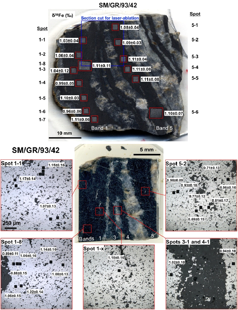
Figure 1: representative sample showing Fe isotope compositions measured by micromilling (top) and fs-LA bottom
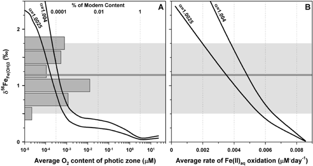
Figure 2. Summary results of dispersion/reaction modeling of the Isua basin assuming production of O2 by oxygenic photosynthesis or Fe oxidation by anoxygenic photosynthetic Fe oxidizers. A) Resulting average photic zone O2 concentrations plotted against the weighted average δ56Fe values of the HFO produced. B) Resulting average rates of Fe(II)aq oxidation in the photic zone plotted against the resulting weighted average δ56Fe values of the HFO produced. The two curves in each panel represent the model results for Fe isotope fractionation factors of Δ56FeHFO-Fe(II) = 1.0025 and 1.0040. The horizontal dark gray line spanning the two panels at δ56Fe = 1.2 ‰ represents the assumed average δ56Fe value for the HFO produced by Fe(II)aq oxidation during Isua BIF deposition. This value was calculated from the average measured magnetite δ56Fe value (0.8 ‰) and the assumption that one-third of the Fe in magnetite (Fe3O4) was provided by addition of Fe(II)aq with a δ56Fe = 0 ‰ to the initial HFO precipitate. The vertical histogram in the left panel represents the data in the present study, converted to the assumed original δ56Fe value of the precipitated HFO in the same manner. The light gray field covers the range of data and is used to guide the eye.
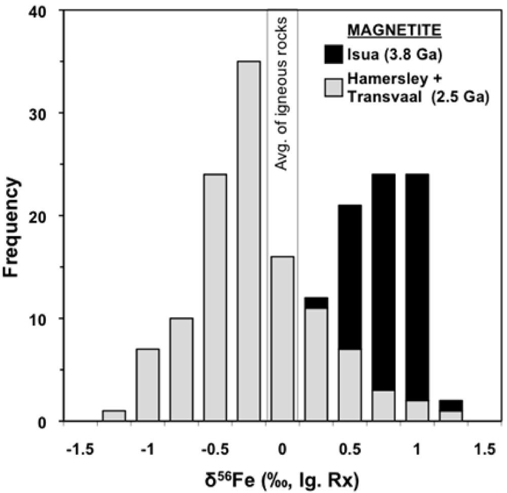
Figure 3. Comparison of BIF magnetite Fe isotope compositions of the 3.8 Ga Isua Supracrustal Belt and 2.5 Ga Hamersley and Transvaal basins. This comparison suggests a fundamental difference in the Fe cycles that produced the BIFs in these two time periods. The peak in δ56FeMt values for the Hamersley and Transvaal basin BIFs is centered just below 0 ‰, distinctly lower than the distribution of δ56Fe values of the Isua BIF. Johnson et al. (2008a) interpret the peak at δ56Fe ~0 ‰ for the 2.5 Ga BIFs to reflect the inheritance of the δ56Fe values of HFO that was produced by complete oxidation of Fe(II)aq whereas Isua δ56FeMt values greater than zero are thought to reflect partial oxidation. Data for Isua BIFs are from the present study and those for the Neoarchean/Paleoproterozoic Hamersley and Transvaal BIFs are from Johnson et al. (2003), Rouxel et al. (2005), Johnson et al. (2008a), and Steinhoefel et al. (2010).
Publications
- Czaja, A.D., Johnson, C.M., Beard, B.L., Roden, E.E. & Li, W. (2012, Submitted). Likely role for limited biological Fe oxidation in 1 the deposition of the 3.7–3.8 Ga Isua banded iron formation determined by multiple scales of Fe isotope analyses. Earth and Planetary Science Letters.
-
PROJECT INVESTIGATORS:
-
PROJECT MEMBERS:
Eric Roden
Co-Investigator
Stephen Moorbath
Collaborator
Andrew Czaja
Postdoc
Weiqiang Li
Postdoc
-
RELATED OBJECTIVES:
Objective 4.1
Earth's early biosphere.

